Tutorial
We being by loading NumPy, PyPlot, SUFTware:
import numpy as np
import matplotlib.pyplot as plt
import suftware as sw

# Enable interactive plotting
plt.ion()
Next we simulate data from a Gamma distribution:
# Generate data from a Gamma distribution
np.random.seed(0)
data = np.random.gamma(shape=5, scale=1, size=100)
To estimate the probability density, do this:
# Perform DEFT density estimation using SUFTware
density = sw.DensityEstimator(data)
This creates an instance of the sw.DensityEstimator class.
The DEFT density estimation algorithm is run as part as part of this
object’s initialization process.
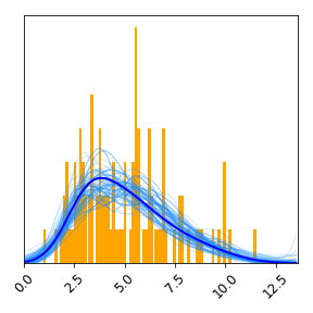
To quickly view the estimated probability density, use density.plot():
# Plot density estimate using built-in plotting routine and save to file
density.plot()
This will create a matplotlib figure resembling the one
below. A histogram of the data is shown in orange, the optimal density estimate
is shown in blue, and plausible densities are shown in light blue.
Because the optional save_as argument is set, this plot is also
saved to a PNG file. Other optional arguments to density.plot() can be used
to specify styling options. See Documentation for more information.
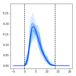
DEFT estimates each probability distribution on a grid contained within
a finite bounding box. Both the bounding box and the grid were
set automatically in this example, but these as well as other grid
characteristics can be set by the user by passing additional parameters to
the DensityEstimator constructor. See Documentation for more
information.
Information about the grid and bounding box are stored in the
attributes of density:
density.bounding_box: Lower and upper edges of the bounding box.density.grid: Locations of the gridpoints used.density.grid_spacing: Distance between neighboring grid points.density.num_grid_points: Number of grid points used.
The values of the optimal density estimate at each grid point are stored
in density.values. The density.evaluate() method allows this density to
be evaluated at any other set of locations. The ensemble of posterior-sampled
densities can be evaluated in a similar manner. Note that all estimated
distributions evaluate to zero outside of the bounding box:
# Create new grid
new_grid = np.linspace(-5,20,10000)

# Evaluate optimal density on new grid
new_values = density.evaluate(new_grid)

# Evaluate sampled densities on new grid
new_sampled_values = density.evaluate_samples(new_grid)

# Create figure
plt.figure(figsize=[4,4])

# Plot optimal and posterior-sampled densities
plt.plot(new_grid, new_sampled_values, color='dodgerblue', alpha=.1)
plt.plot(new_grid, new_values, color='blue')

# Draw lines indicating bounding box
plt.axvline(density.bounding_box[0], linestyle='--', color='black')
plt.axvline(density.bounding_box[1], linestyle='--', color='black')

# Show plot
plt.tight_layout()
plt.savefig('tutorial_2.png')
plt.show()
See Documentation for more information on the SUFTware API.